“Statistics 101”—A Primer for the Genetics of Complex Human Disease
Adapted from Genetics of Complex Human Diseases (ed. Al-Chalabi and Almasy). CSHL Press, Cold Spring Harbor, NY, USA, 2009.Abstract
This article reviews the basis of probability and statistics used in the genetic analysis of complex human diseases and illustrates their use in several simple examples. Much of the material presented here is so fundamental to statistics that it has become common knowledge in the field and the originators are no longer cited (e.g., Gauss).
SET THEORY BASICS
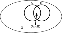
To start, we need to briefly review the set theory basics that apply to genetics analysis. Let the entire event space be denoted by Ω and the null space (or empty set) by Ø. Let A and B be two events that are both elements of Ω. The symbol ∩ denotes “and” or “intersection” (Fig. 1) and the symbol ∈ indicates when an event is a member, or element, of a set. The outcomes A and B are mutually exclusive when A ∩ B = Ø. If A ∈ Ω, then the complement of A (not A), which is denoted as 〈Ā〉, is also an element of Ω. The symbol ∪ denotes “or” or “union.” Our final rule here is that, if A ∈ Ω and B ∈ Ω, then A ∩ B ∈ Ω.
PROBABILITY THEORY IN GENETIC ANALYSIS
We can now move on to the probability of an event or set of events. Let P(A) denote the probability of outcome A, in which A can be a single event or a set of events. Likewise, let P(B) denote the probability of outcome B. The probability of both outcomes A and B occurring is denoted by P(A ∩ B) or P(A, B). The probability of outcome A or outcome B occurring is P(A ∪ B). The basis of probability comes from the following four rules: (a) P(Ω) = 1; (b) P(Ø) = 0; (c) 0 ≤ P(A) ≤ 1; and (d) if A ∩ B = Ø, then P(A ∪ B) = P(A) + P(B). These four rules can be used in combination to provide more probabilistic insights. As an example, the probability of
 can be derived as follows: P(Ω) = 1, so
  . These events are mutually exclusive so
  and finally
  .
.
Conditional Probability
The concept of conditional probability plays an important role in genetic analysis. The conditional probability of event A
given event B is

Conditional probabilities can be particularly useful when it is difficult to calculate P(A) directly. Using this notation, we can express the probability of A in terms of joint or conditional probabilities,

Here, outcome A is partitioned into two parts by the two outcomes B and  . We can extend this partitioning to any number of outcomes.
Bayes’ theorem also relies on conditional probability. Suppose it is difficult to calculate P(B | A) directly; however, P(B),  , and
, and  can be calculated. By Bayes’ theorem,

Again this theorem can be extended to more than the two outcomes B and  .
.
Independence
Another important concept is independence. If A and B are independent, then P(A ∩ B) = P(A)P(B). If P(B) > 0, then, using the definition of conditional probability, independence can be expressed as P(A | B) = P(A). Intuitively then, independence between events A and B means that knowing that B occurred does not change the probability of A occurring.
Example: Linkage Equilibrium
A haplotype is a set of alleles at genes inherited from the same parent. Two loci C and D, which make up part of a haplotype, are in linkage equilibrium if the haplotype frequency equals the product of the allele frequencies. That is P(ci, dj) = P(ci)P(dj) for any allele ci at C and any allele dj at D. So, linkage equilibrium is an example of independence. When a haplotype frequency is not equal to the product of the corresponding allele frequencies, then these loci are in linkage disequilibrium (LD; for more information on LD, see Genome-Wide Association Studies [Al-Chalabi 2009]).
Example: Hardy–Weinberg Equilibrium
For a specified locus, the Hardy–Weinberg law (p2 + 2pq + q2 = 1) allows us to calculate genotype frequencies in terms of the allele frequencies (Hardy 1908; Weinberg 1908). If there is a very large population size, no mutation, no selection, and random mating with respect to the locus, then the Hardy–Weinberg law dictates that the genotype frequencies in a population remain constant from generation to generation and the expected genotype frequencies can be derived from the expected allele frequencies (Hardy–Weinberg equilibrium, HWE). As an example, consider the blood group MNc. If allele M has population frequency p and allele N has frequency q, then under HWE we can calculate the genotype frequencies. The genotype M/N is an unordered genotype that is shorthand for the union of the two ordered M|N and N|M genotypes (the parental origin of the alleles is known). That is, M/N denotes the event that the M is from the mother and the N is from the father or that the N is from the mother and the M is from the father. The two ordered genotypes are mutually exclusive, so using our probability rules we know that P(M/N) = P(M from mother, N from father) + P(N from mother, M from father). Random union of gametes implies independence so P(M/N) = pq + qp = 2pq. Similarly, we can show that P(M/M) = p2, and P(N/N) = q2 under HWE.
Example: Determining the Frequency of ABO Blood Type by Affection Status
Clarke et al. (1959) provide blood types for 521 individuals suffering from duodenal ulcers and 680 unaffected controls. Lange (2002) summarized the data from the ulcer patients, noting that there were 186 with blood type A, 38 with blood type B, 13 with blood type AB, and 284 with blood type O, and for the controls, there were 279 with blood type A, 69 with blood type B, 17 with blood type AB, and 315 with blood type O.
The frequency of blood type O in those individuals with ulcers is the conditional probability

Likewise the frequency of blood type O in the unaffected individuals P(O | Unaffected) = 315/680 = 0.465. Note that these probabilities are not the same as the probability of having an ulcer given blood type O, P(Ulcer | O) = 0.474, or the probability of not having an ulcer given blood type O, P(Unaffected | O) = 0.526. Assuming HWE and an iterative gene counting algorithm, which is an example of an expectation–maximization (E–M) algorithm (see Lange 2002), provides the allele frequencies for ulcer patients and the allele frequencies for unaffected controls (P(O | Ulcer) = 0.7363, P(A | Ulcer) = 0.2136, P(B | Ulcer) = 0.0501, P(O | Unaffected) = 0.6853, P(A | Unaffected) = 0.2492, P(B | Unaffected) = 0.0655).
VARIABLES, PARAMETERS, AND DISTRIBUTIONS IN GENETIC ANALYSIS
We start with a few definitions. A random variable is something we can measure, control, or manipulate in research. Examples
include continuous values like high-density lipoprotein cholesterol levels or discrete values like disease status. A parameter
is any characteristic of a population and a statistic is any characteristic of a sample. Some common parameters for a continuous
random variable X are its population mean, µx, population variance,  , and population standard deviation, σx. The relationship between two continuous random variables X and Y can be summarized by their population covariance, σxy. Some common measures for a dichotomous categorical trait include the proportion and its variance. The data are assumed to
be generated from some underlying probabilistic model. This model defines the range of possible values and how likely they
are and is called the theoretical distribution. For a random variable X, the probability density is f(x) = P(X = x) for all allowable values x and the cumulative probability distribution is F(x) = P(X ≤ x).
Often we cannot directly observe a parameter, and so we use a statistic calculated on a sample to estimate the parameter value
and make inferences concerning the population. The observed data from the sample make up the observed distribution. The parameters
µ,  , σx, σxy are estimated by the sample mean
 sample variance
 sample standard deviation
 and sample covariance
 in which n is the number of individuals in the sample. Another important parameter is the population correlation coefficient, ρ = σxy/σxσy, which is a standardized covariance between two continuous variables. The population correlation is estimated by the sample
correlation coefficient r, which is calculated as r = covxy/sdxsdy.
We are often interested in whether the observed distribution could have been drawn from a putative theoretical distribution. We can get a handle on whether this hypothesis is true by determining whether a statistic value for a sample is consistent with a parameter value that is calculated from the putative theoretical distribution.
Theoretical probability distributions depend on whether the variable is discrete or continuous. There are a number of theoretical distributions that pop up frequently in genetic analysis. These distributions include the uniform, the binomial, the normal, and the chi-square. Rather than concentrate too heavily on their formulas, we will examine them intuitively and point out their most important features.
Discrete Uniform Distribution
Let there be a finite number of possible outcomes W; each are equally probable (with the probability of a specific outcome being 1/W). If there are n total observations from a uniform distribution, we expect n/W of these observations to be in each of the possible categories with variance (n/W)(1 – 1/W). The discrete uniform distribution is found in genetic analysis when quantifying prior beliefs in which there is little or no real evidence to support one hypothesis more than another. As an example, suppose gene mapping has narrowed down the location of a disease conferring mutation to a chromosomal region containing 20 genes. Without additional biological information, it may be a good starting point to suppose that the probability that any one of these genes contains the mutation is 1/20, that is, to assume a discrete uniform distribution.
Normal Distribution
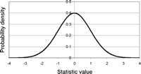
The normal distribution is defined for continuous data (data that can take on any value). The probability density is a bell-shaped curve that is symmetric and defined for the whole real line (Fig. 2). Because the density is symmetric and unimodal, the mean, the 50th percentile (median), and the mode (the peak) all have the same value. The bigger σx is, the greater the spread of the density. The normal density has inflection points (points in which the second derivative is 0) at µx − σx and µx + σx. Because the data are continuous, the probability of getting exactly the value x is 0. The probability that the value is less than or equal to x is always positive (the cumulative distribution). Likewise the probability that the value is greater than x is always positive. Many of the methods that are used to map quantitative trait loci (e.g., variance component methods for gene mapping [see as examples, Amos 1994; Almasy and Blangero 1998; Bauman et al. 2005]) use models that implicitly assume that the trait or a transformation of the trait has a distribution that is normal or is a mixture of normal distributions.
The standard normal density. Shown is an example of the normal density with µ = 0 and σ = 1 (the standard normal density).
The normal distribution is particularly important in statistics because, by the central limit theorem, it is the theoretical
distribution of the sampling mean  . More precisely, as the sample size used to calculate
  increases, the shape of the sampling distribution of
  approaches a normal distribution with mean µx and standard deviation σx/√n.
Chi-Square Distribution
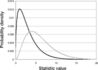
Another important distribution in genetic analysis is the chi-square distribution. The chi-square distribution is defined for continuous data. If Y is the sum of the squares of N independent variables Xi(i = 1, …, N) in which each Xi has a normal density with µ = 0 and σ = 1 (each has a standard normal density), then Y has a chi-square distribution. The shape of the density depends on N (Fig. 3). Because Y is a sum of squared values, Y can never be less than 0. However, Y can be arbitrarily large. Often we assume that a goodness-of-fit comparison of observed and expected results follows a chi-square distribution for categorical data, even though the statistic takes on discrete values. This approximation is reasonable provided we have enough data. Chi-square approximations show up in the contingency table analyses that examine the question of whether genotype frequencies are associated with disease status.
Binomial Distribution
The binomial distribution is also defined for discrete data. Suppose that there are n independent trials and two possible outcomes, success and failure. Then the probability of exactly s successes (the probability density function) is
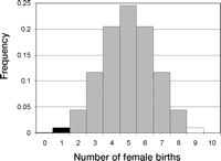
 in which p is the probability of a single success. The terms ps(1 – p)n–s are present because each of the s successes and n – s failures is independent and so their probabilities multiply. The term n!/(n – s)!s! is the number of ways that these s successes and n – s failures can be arranged. The density is unimodal but not usually symmetric. When p = 1/2 the density is symmetric (Fig. 4), but when p < 1/2 the mode of the density is skewed toward low values of s and when p > 1/2 the mode of the density is skewed toward high values of s. The probability of at least s successes (the cumulative distribution) sums the probability densities for 0 to s,

Example of a binomial density and a graphical depiction of a one-sided p value and a two-sided p value. The density is binomial with p = 1/2. The x axis denotes the number of births. There can be 0 to 10 births. Although difficult to see in the graph for the values 0 and 10, each of the 11 possible outcomes has nonzero probability and is represented by a histogram block. The area defined by the black blocks at 0 and 1 represent the p value for the one-sided test. The area represented by the black blocks at 0 and 1 and the white blocks at 9 and 10 represent the p value for the two-sided test.
The binomial distribution and its generalization for multiple possible outcomes, the multinomial distribution, underlie a number of statistical genetic tests. The probability of s affected offspring from a random sample of n independent affected–unaffected matings provides a classic example from segregation analysis (Sham 1998).
MAXIMUM LIKELIHOOD ESTIMATION
A likelihood LH is proportional to the probability of the data given the hypothesis H, in which the constant of proportionality is arbitrary. We can think of a likelihood as a surface (a function) whose height varies with the parameter values but the data stay fixed. Therefore, maximum likelihood estimation finds the parameter values that best fit the observed data. These values are called the maximum likelihood estimates (MLEs) of the parameters. Because the logarithm is a monotonic transformation (the logarithm preserves inequalities among the y values, i.e., if y1 < y2, then ln(y1) < ln(y2)), the MLEs for the likelihood are also the MLEs for natural logarithm of the likelihood (log-likelihood). MLE has several desirable properties. MLEs are often not too difficult to calculate (at least numerically), they are consistent estimates (as the sample size increases the estimate gets better), and they are asymptotically unbiased (expected value of the MLEs equals the true parameter values, at least when the sample size approaches infinity).
The log-likelihood tends to be easier and more stable to maximize. When the number of parameters is small and the log-likelihood amenable, we can maximize the log-likelihood analytically. However, most of the time we maximize the log-likelihood numerically. When the log-likelihood has multiple maxima (i.e., a surface with multiple hills and valleys) and there are a number of parameters, it can be tricky to find the global maximum. To help find the global maximum, it is useful to try several initial values for the estimates when implementing the maximization algorithm.
Example: Maximum Likelihood Estimation for Female Births
Suppose we want to estimate the number of female births in n independent births. We assume that the distribution is binomial with s successes in n trials and the probability of a female at any given birth is p. The likelihood is then L(p | s, n) = kps(1 – p)n–s in which k is an arbitrary positive constant that does not depend on p. Here the maximum of the likelihood represents the point in the likelihood surface that has a slope of 0 and has negative
curvature. In this case, the maximum can be found by setting the first derivative of the log-likelihood equal to 0 and solving
for p. The MLE is  , which is the observed proportion of female births. Any other value
  will lead to a lower value for the likelihood. For example, let s = 3 and n = 10, then
  and
and  . When
  ,
,  and when
 .
.
HYPOTHESIS TESTING PROVIDES CONFIDENCE IN A RESULT
Along with estimation, we want some measure of confidence in our result. Hypothesis testing is a very common way to provide this confidence. Hypothesis testing starts with a research hypothesis and a contradictory explanation. The contradictory explanation is the null hypothesis H0, and the research hypothesis (the hypothesis we often believe is the truth) is the alternative hypothesis Ha. The purpose of the hypothesis test is to support or refute H0. H0 will be rejected or will fail to be rejected depending on the value of a test statistic. If the test statistic is very unlikely given H0 is true, then H0 is rejected. The decision made to reject or not to reject H0 falls into one of four possible cases. There are two possible correct decisions: (1) H0 was not rejected and H0 is actually true or (2) H0 was rejected and Ha is actually true. There are two possible incorrect decisions: (1) type I errors (false positives) in which H0 was rejected but H0 is actually true or (2) type II errors (false negatives) in which H0 was accepted but Ha is actually true. Although the stochastic nature of data dictates that a correct decision cannot be made all the time, a desirable hypothesis testing procedure has both low type I and type II error rates.
p Values
As part of a hypothesis test, we determine how unusual a test statistic is if H0 is true. One such measure is the p value, which is the probability of a test statistic that is as extreme or more extreme than the observed test statistic if H0 is true. Before applying a test, a significance level (α) should be designated. The significance level is a cutoff, and H0 is rejected if the p value is less than α. In other words, H0 is rejected when the p value is considered too small to have occurred by chance under H0, in which too small is defined by being less than a prechosen α. The significance level depends on how willing we are to make a type I error, and, although there are some popular values, the value of α is an arbitrary matter of choice. See Multiple Testing and Power Calculations in Genetic Association Studies (So and Sham 2011) for more discussion of type I and type II error rates and significance thresholds in the context of power and multiple testing in association studies.
Before moving on to an example, there are a few caveats regarding p values that deserve mention. First, the p value is not the same as the posterior probability that the null hypothesis is true, P(H0 | data). Second, just because a p value is small it does not mean that the null hypothesis is impossible. As an example, a p value of 0.05 means that if we repeated the experiment 100 times and the null hypothesis is true, then we would expect to see data as extreme or more extreme than observed 5 of the 100 times. This relates to our final caveat, if multiple experiments are performed, then the rejection of any individual test must be made less frequent if an overall experimental-wide α is desired. That is, we need to take into account multiple testing in our decision-making process. Some researchers advocate monitoring the expected proportion of false rejections of H0 among all rejections, the false discovery rate (Benjamini and Hochberg 1995).
Example: Female Births
Suppose we want to determine if females are less likely to be born than males in a population. Our null hypothesis (H0) is p = 1/2, and in this case our alternative hypothesis, Ha, is p < 1/2 (a one-sided test). We collect data on 10 births (too small a sample size in practice but useful for this illustration). The null distribution is binomial, with 10 trials and p = 1/2. Let α = 0.05. The test statistic is the number of female births (s). We find that only 1 of these 10 children are female (s = 1). Test statistics as extreme or more extreme for this one-sided test are s = 1 and s = 0. The p value is 0.01074 (Fig. 4).
Alternatively, we could have conducted a two-sided test. The research question is whether the probability of a female birth differs from the probability of a male birth. H0 remains p = 1/2, but Ha is now p ≠ 1/2, so that too many or too few female births are cause for rejection of the null hypothesis. The observed data remain 1 female birth out of 10 births. The null distribution is still binomial with 10 trials and p = 1/2, but now test statistics that are as extreme or more extreme than the observed test statistic are 0, 1, 9, and 10 and the p value is 0.02148 (Fig. 4).
Example: Association between ABO Blood Type and Ulcer Susceptibility
We return to the Clarke et al. (1959) data. The null hypothesis here is that there is no association between ABO blood type and duodenal ulcers. This is equivalent
to a hypothesis of independence—that the joint probability of ABO blood type and ulcer status can be calculated as the product
of the marginal probability of ABO blood type and the marginal probability of ulcer status. The alternative hypothesis is
that the ABO blood type and duodenal ulcers are associated. Let α = 0.05. We now need to specify the test statistic and its
distribution under the null hypothesis. Let Nij be the number of individuals with blood type i and affection status j, let Nj be the number of individuals with affection status j, let Ni. be the number of individuals with blood type i, and let N. be the total number of individuals in the study. Then the expected number of individuals with blood type i and affection status j is
 under the null hypothesis of no association. As an example, the expected number of individuals with type A blood and ulcers
is
 which is different from the observed number (186). But could this difference be caused by chance alone or is there evidence
of an association? A statistic that measures the relative difference between the observed number of individuals with each
blood type and affection status from their expected values is

When there is no association (under the null hypothesis), t has an asymptotically chi-square distribution with three degrees of freedom (df). Using the Clarke et al. (1959) data, t = 8.824. The probability of a t that is greater than or equal to 8.824 under the null hypothesis of no association (the p value) is 0.0317. Thus, we reject the null hypothesis and conclude that there is evidence for an association between ABO blood type and ulcer susceptibility.
Likelihood Ratios, Likelihood Ratio Test Statistics, and Logarithm of the Odds Scores
Often hypothesis testing uses a likelihood ratio (LR). We can compare the likelihood for different models or hypotheses by
calculating the likelihood ratio, LR = LH1/LH2, in which LH1 is the likelihood for hypothesis 1 and LH2 is the likelihood for hypothesis 2. When LR > 1, the data are more likely under H1 than under H2, and, when LR < 1, the data are more likely under H2 than under H1. Often, as in our female birth example, we do not have a simple alternative hypothesis. We can also form a LR for a null
hypothesis whose state space is nested within a larger hypothesis space. Let θ denote the parameters, Ω0 denote the null hypothesis space for these parameters, and ΩA denote the alternative space. Let these two spaces be mutually exclusive (Ω0 ∩ ΩA = Ø). Then the likelihood ratio compares the maximum of the likelihood for the union of the spaces to the maximum of the
likelihood for just the null space,

Notice that now LR ≥ 1.
Twice the natural logarithm of the likelihood ratio is called the likelihood ratio test statistic (LRT). The dfs depend on the number of additional parameters maximized in Ha versus H0. Under the null hypothesis, the distribution of the LRT is often (but not always) asymptotically chi-square with these dfs (Self and Liang 1987). A logarithm of the odds (LOD) score is similar to the LRT, except that a LOD score is the base 10 logarithm of the LR.
Example: Hypothesis Testing Using an LRT for Female Births
Rather than using the binomial distribution, we can conduct a hypothesis test using the LRT assuming that, under H0, the LRT has an asymptotic chi-square distribution with df = 1. As before, let α = 0.05 and let the test be two-sided. H0 is p = 1/2 and Ha is p ≠ 1/2. The likelihood under H0 is

The maximum likelihood under Ha is

LR = 39.682, LRT = 7.3613, and the p value = 0.00666. Note that this p value from the large sample approximation to the distribution differs from the p value we calculated assuming that the data came from a binomial distribution (0.02148). When the sample size is small, we are better off using the exact p value derived from using the binomial distribution rather than relying on an asymptotic approximation.
Power
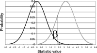
The power of a test is the probability of rejecting the null hypothesis given an alternative hypothesis is true. Power and the probability of a type II error (β) sum to 1. Power depends on the sample size and the specifications of the alternative hypothesis. Power also depends on the maximum type I error that can be tolerated, the significance level. Holding everything else constant, the smaller α is, the lower the power and correspondingly the greater the chance of a type II error (Fig. 5).
Graphical depiction of the null and alternative densities. The black curve represents density under the null hypothesis and the gray curve represents the density under the alternative hypothesis. The vertical line at 2.32 marks the boundary of the one-sided significance level (α = 0.01, area to the right of the line under the null density curve) and the type II error (β = 0.19, area to the left of the line under the alternative density curve). The power is 0.81.
Whenever possible, power estimations should be performed before embarking on a genetic analysis because they will produce information relevant to study design. As an example, the relative power of various genome-wide association study (GWAS) designs can be compared and balanced against the type I error rates. Reducing the significance level will reduce the number of false inferences of association, but it may produce unacceptable decreases in power in a GWAS. In such circumstances, one possible approach is to modify the overall nature of the testing, accepting that false positives will be generated if the “true” results are also to be found, and then seeking replication to distinguish between the true and false results. How to optimize GWAS designs is an active area of research (e.g., see Dudbridge et al. 2006; Elston et al. 2007; Kraft and Cox 2008; Moskvina and Schmidt 2008).
- © 2011 Cold Spring Harbor Laboratory Press


